Beyond the Blur: Understanding the Power and Perils of Data Smoothing
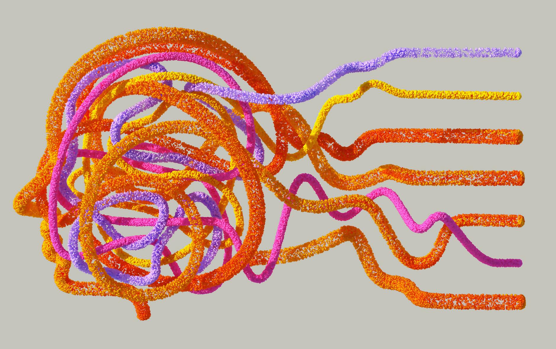
In a world awash with data, the raw signal is often obscured by noise. Whether you’re analyzing financial markets, tracking scientific experiments, or monitoring public health trends, the inherent variability and random fluctuations can make it difficult to discern meaningful patterns. This is where the crucial technique of smoothing comes into play. Smoothing is not merely about making data look prettier; it’s a fundamental analytical tool that helps reveal underlying trends, reduce the impact of outliers, and improve the interpretability and predictive power of datasets. Understanding why and how to smooth data is essential for anyone seeking to extract actionable insights from complex information.
Why Data Smoothing is Indispensable for Insight
The core purpose of data smoothing is to reduce the random variations, or “noise,” present in a dataset. This noise can arise from various sources, including measurement errors, inherent stochasticity of a system, or simply the granular nature of the data collection process. Without smoothing, these fluctuations can:
- Mask true trends: A genuine upward or downward movement might be obscured by short-term ups and downs.
- Lead to misinterpretations: Analysts might mistake random spikes for significant events or dismiss minor changes as inconsequential.
- Degrade model performance: Machine learning models trained on noisy data are more prone to overfitting, meaning they learn the noise as if it were signal, leading to poor generalization on new data.
- Hinder forecasting: Predicting future behavior becomes unreliable when the past is dominated by unpredictable volatility.
Who should care about smoothing? The answer is broad:
- Financial Analysts: To identify long-term stock market trends, economic cycles, or volatility patterns, moving averages are indispensable.
- Scientists and Researchers: To highlight genuine experimental results amidst measurement uncertainty, signal processing techniques like filtering are vital.
- Public Health Officials: To track disease outbreaks and understand epidemiological trends without being misled by daily reporting variations.
- Engineers: To monitor sensor readings and system performance, identifying gradual degradation or anomalies.
- Business Intelligence Professionals: To understand sales performance, customer behavior, and operational efficiency over time.
- Data Scientists and Machine Learning Engineers: As a preprocessing step to improve model robustness and interpretability.
The Historical Roots and Evolution of Smoothing Techniques
The concept of smoothing is as old as the practice of data analysis itself. Early methods were often intuitive and visually driven, akin to drawing a “best-fit” line through a scatter plot.
Historically, simple techniques like the moving average have been foundational. First described in statistical literature for economic data, moving averages involve calculating the average of a subset of data points over a defined period. This method smooths out short-term fluctuations by averaging them out over the window.
As computational power grew, more sophisticated methods emerged. The development of statistical theory provided a rigorous framework for understanding noise and signal. Techniques like exponential smoothing, first popularized by Robert G. Brown in the 1950s, offered a more adaptive approach by giving more weight to recent observations, making it responsive to changing trends. This was particularly impactful in inventory control and forecasting applications.
In signal processing and image analysis, concepts like convolution became central. This mathematical operation allows for the application of various smoothing kernels (e.g., Gaussian, Savitzky-Golay) to data. The Savitzky-Golay filter, for instance, fits polynomial functions to subsets of data points, preserving features like peak height and width better than simple moving averages, which can sometimes distort or flatten them. These advancements enabled smoother, more interpretable signals from complex sources like seismic data or medical imaging.
More recently, with the rise of machine learning, techniques like LOESS (Locally Estimated Scatterplot Smoothing) and spline smoothing have gained prominence. LOESS fits simple models to localized subsets of the data, allowing for flexible, non-linear smoothing. Splines use piecewise polynomial functions to create smooth curves that pass through or near the data points, offering a highly adaptable approach to capturing complex underlying patterns.
Deep Dive: A Spectrum of Smoothing Methodologies
Smoothing techniques can be broadly categorized based on their underlying principles and mathematical approaches. Each offers a unique balance of simplicity, computational efficiency, and ability to preserve data characteristics.
Simple and Intuitive Approaches
These methods are easy to understand and implement, making them excellent starting points.
- Moving Average (MA): The most straightforward method. A window of a fixed size slides across the data, and the average of the points within that window is calculated.
- Simple Moving Average (SMA): All points in the window have equal weight.
- Weighted Moving Average (WMA): Assigns different weights to data points within the window, often giving more importance to recent data.
- Exponential Smoothing (ES): Assigns exponentially decreasing weights to older observations. More recent data points have a higher weight.
- Simple Exponential Smoothing (SES): Suitable for data without a trend or seasonality.
- Holt’s Linear Trend Method: Extends SES to handle data with a trend.
- Holt-Winters’ Seasonal Method: Further extends Holt’s method to incorporate seasonality.
Frequency Domain and Kernel-Based Smoothing
These methods leverage mathematical operations to filter out high-frequency noise.
- Fourier Transform-Based Smoothing: Data is transformed into the frequency domain, where high-frequency components (often associated with noise) can be attenuated or removed, and then transformed back to the time domain.
- Savitzky-Golay Filter: This method fits a polynomial to a rolling window of data points and uses the polynomial to estimate the smoothed value. It’s known for preserving the shape and height of peaks better than simple moving averages.
- Kernel Regression (e.g., Nadaraya-Watson): This non-parametric technique uses a kernel function to assign weights to neighboring data points, effectively averaging them based on their proximity to the point being smoothed.
Advanced and Adaptive Techniques
These offer greater flexibility and can adapt to complex data patterns.
- LOESS (Locally Estimated Scatterplot Smoothing): A non-parametric regression method that fits simple models (typically linear or quadratic polynomials) to localized subsets of the data. The smoothness is controlled by a span parameter, which determines the proportion of data used for each local fit.
- Spline Smoothing: Uses piecewise polynomial functions (splines) to create a smooth curve that approximates the data. A penalty term is often included to control the degree of smoothness, balancing fit to the data with the complexity of the curve.
- Kalman Filter: A recursive algorithm that estimates the state of a dynamic system from a series of noisy measurements. It’s particularly powerful for time-series data where the underlying system evolves over time. The Kalman filter provides an optimal estimate in a mean-squared error sense.
The Tradeoffs and Limitations: When Smoothing Goes Wrong
While smoothing is powerful, it’s not a panacea. Misapplication can lead to significant distortions and misleading conclusions. Awareness of these limitations is critical.
Information Loss and Distortion
- Loss of Detail: The very act of smoothing removes high-frequency variations. This can be detrimental if these variations contain important information, such as sharp spikes indicating critical events or rapid changes.
- Attenuated Peaks and Valleys: Simple smoothing methods like moving averages can flatten peaks and widen troughs, making it harder to identify the true magnitude or timing of extreme events.
- Lag: Moving averages, especially simple ones, inherently lag behind the actual data. This means the smoothed trend will appear later than the real shift in the data, which can be problematic for real-time decision-making.
- Distortion of Autocorrelation: Smoothing can alter the temporal dependencies within a dataset, impacting subsequent time-series analyses.
Parameter Sensitivity and Choice
The effectiveness of most smoothing techniques hinges on the correct selection of parameters:
- Window Size/Span: In moving averages and LOESS, this determines the degree of smoothing. A small window captures more detail but is noisier; a large window is smoother but might obscure trends.
- Kernel Function: The shape of the kernel in kernel regression can influence the results.
- Polynomial Degree (Savitzky-Golay, Splines): The order of the polynomial fitted affects how well it captures local curvature.
- Damping Factors (Exponential Smoothing): Choosing appropriate alpha, beta, and gamma values is crucial for accurate forecasting.
Incorrect parameter choices can lead to under-smoothing (still too noisy) or over-smoothing (too much detail lost).
Assumptions and Model Fit
- Model Misspecification: Techniques like exponential smoothing and Kalman filters rely on underlying assumptions about the data generation process (e.g., linearity, stationarity). If these assumptions are violated, the smoothing and resulting forecasts can be biased.
- Outlier Amplification: While smoothing aims to reduce outlier impact, poorly chosen methods or extreme outliers can sometimes be amplified or create artifacts in the smoothed series.
Computational Cost
While simple methods are computationally inexpensive, more advanced techniques like LOESS or certain spline smoothing methods can be computationally intensive, especially for very large datasets.
Practical Guidance: Applying Smoothing Wisely
To effectively leverage smoothing, follow a systematic approach:
- Understand Your Data and Objective: Before applying any technique, deeply understand the nature of your data and what you aim to achieve. Are you looking for long-term trends, short-term fluctuations, or anomaly detection? The objective dictates the appropriate method and parameters.
- Visualize Before and After: Always plot the raw data alongside the smoothed data. This visual comparison is the most immediate way to assess if the smoothing is achieving the desired effect without undue distortion.
- Experiment with Different Methods and Parameters: Don’t settle for the first method you try. Compare the results of several techniques (e.g., SMA vs. exponential smoothing vs. LOESS) and vary parameters (window size, span) to see which best reveals the underlying signal while preserving essential features.
- Consider the Tradeoffs: Be acutely aware of what you might be losing. If peak detection is critical, avoid overly aggressive smoothing. If lag is a concern, consider adaptive methods or simpler, less laggy techniques.
- Validate Your Smoothed Data: If the smoothed data is used for forecasting or as input to a model, validate the performance of that downstream task. Does smoothing improve predictive accuracy or model robustness?
- Document Your Process: Clearly record the smoothing method, parameters, and justification for their choice. This ensures reproducibility and transparency.
- Beware of Overfitting with Smoothing: Just as models can overfit data, smoothing can also be “overfit.” A curve that perfectly hugs noisy data points without capturing a genuine trend is overly complex and may not generalize well.
Key Takeaways for Effective Smoothing
- Purpose-Driven: Smoothing should serve a clear analytical objective, not just aesthetic improvement.
- Toolbox Approach: No single smoothing method is universally best. Select based on data characteristics and goals.
- Visual Validation: Always compare raw and smoothed data visually to assess effectiveness and identify distortions.
- Parameter Prudence: Careful selection and tuning of smoothing parameters are crucial.
- Information Cost: Understand that smoothing inherently involves some loss of detail; weigh this against the benefit of noise reduction.
- Reproducibility: Documenting the smoothing process is vital for transparent and repeatable analysis.
References and Further Reading
- NIST Engineering Statistics Handbook: Smoothing Data
A comprehensive overview of various smoothing techniques, their applications, and statistical underpinnings.
https://www.itl.nist.gov/div898/handbook/fpe/section3/fpe33.htm - Brown, R. G. (1959). Statistical forecasting, a view from the command post.
A seminal work introducing exponential smoothing for forecasting and inventory control.
(Note: Full PDF access may require institutional subscription; often cited in statistical texts). - Stone, C. J. (1977). Consistent Nonparametric Regression and Distribution Function Estimation.
Introduces theoretical underpinnings for kernel smoothing methods.
https://projecteuclid.org/journals/annals-of-statistics/volume-5/issue-5/Consistent-Nonparametric-Regression-and-Distribution-Function-Estimation/10.1214/aos/1176344042.full - Hastie, T., Tibshirani, R., & Friedman, J. (2017). The Elements of Statistical Learning: Data Mining, Inference, and Prediction.
Chapter 6 covers smoothing methods in detail, including LOESS and splines.
https://hastie.su.domains/ElemStatLearn/ - Savitzky, A., & Golay, M. J. E. (1964). Smoothing and Differentiation of Data by Simplified Least Squares Polynomials.
The original paper describing the Savitzky-Golay filter.
https://pubs.acs.org/doi/pdf/10.1021/ac60214a047


